On February 20th, Steve Brierley spoke at The Royal Society during a conference focused on the future of quantum computing, networking, and sensing systems. Below is a transcript of his talk.
Quantum computers need massive classical computers to run. In this talk, I'm going to explain why that is. What are these classical computers doing? I’ll also explain some of the constraints that make this a really interesting problem. Then, I'll touch on some of the progress that's been made in this direction over the last few years.
Let's start with classical computing.
Classical computers are essentially a bunch of switches. Transistors switch voltages and we're now very good at making them incredibly small. This is how you implement logic on a classical computer. You're flicking some switches.

Quantum computers look quite different.
Here are two pictures of two different types of quantum computer:
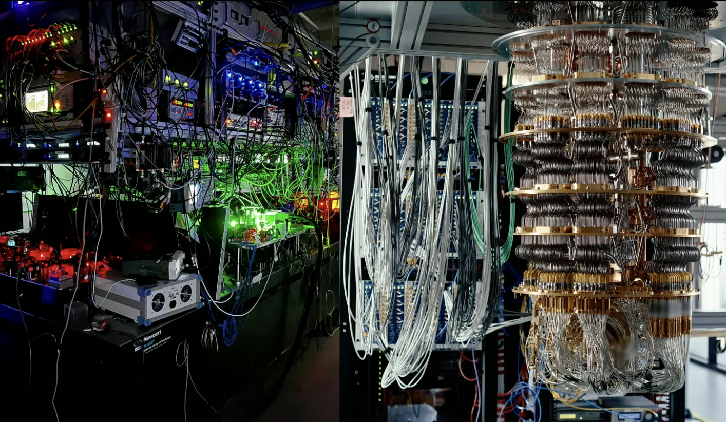
On the left-hand side, you have an AMO system, a neutral atom system in this case. Other systems, like ion traps, look quite similar. On the right-hand side, you can see a solid-state system. In this case, a superconducting one. Again, silicon systems will look pretty similar to this.
What I wanted to call out is that we often see pictures like this with a huge, beautiful chandelier or some lasers on an optical table. What I wanted to draw your attention to is the electronics that are sat next to these computers. What they're doing is generating microwave signals. This is how we control a quantum computer.
Before I talk about those electronics, what are these quantum computers really doing?
These are quite small quantum computers in both cases. We're talking around 100 physical qubits. You can see that you need quite a lot of control electronics, even for that number of qubits. We need to get to hundreds of thousands, if not millions of physical qubits. So, scaling this up is going to be a really interesting problem.
Of course, we'll also need to develop some amazing physics, material sciences, refrigeration, and other technologies but we also need to build some classical electronics. And that's the focus of this talk.
What is this classical system actually doing? Most of it is implementing quantum error correction.
There's a nice plot here from a paper in 2017 that shows the total instruction bandwidth in a quantum computer as you scale up the number of qubits. It's on a log scale, and we're getting to 10^14 or 10^15 operations on this graph. Most of those operations are implementing quantum error correction.

Just to give you a sense of where we're going here, the total number of operations or the amount of data that's coming out of the quantum computer as we get to millions of physical qubits is on the order of 100 terabytes per second, which is similar to Netflix’s global streaming.
So, if we go back a step, we're going to need to build a quantum computer and, next to it, a classical computer that's going to be processing the same amount of data as Netflix currently does worldwide.
This is the scale of the challenge.
One of the reasons that this is interesting is that it's not just the amount of compute that matters, it's also the timescales that you have to solve those computational problems.
Let's think about the timescales of the classical compute across the stack.
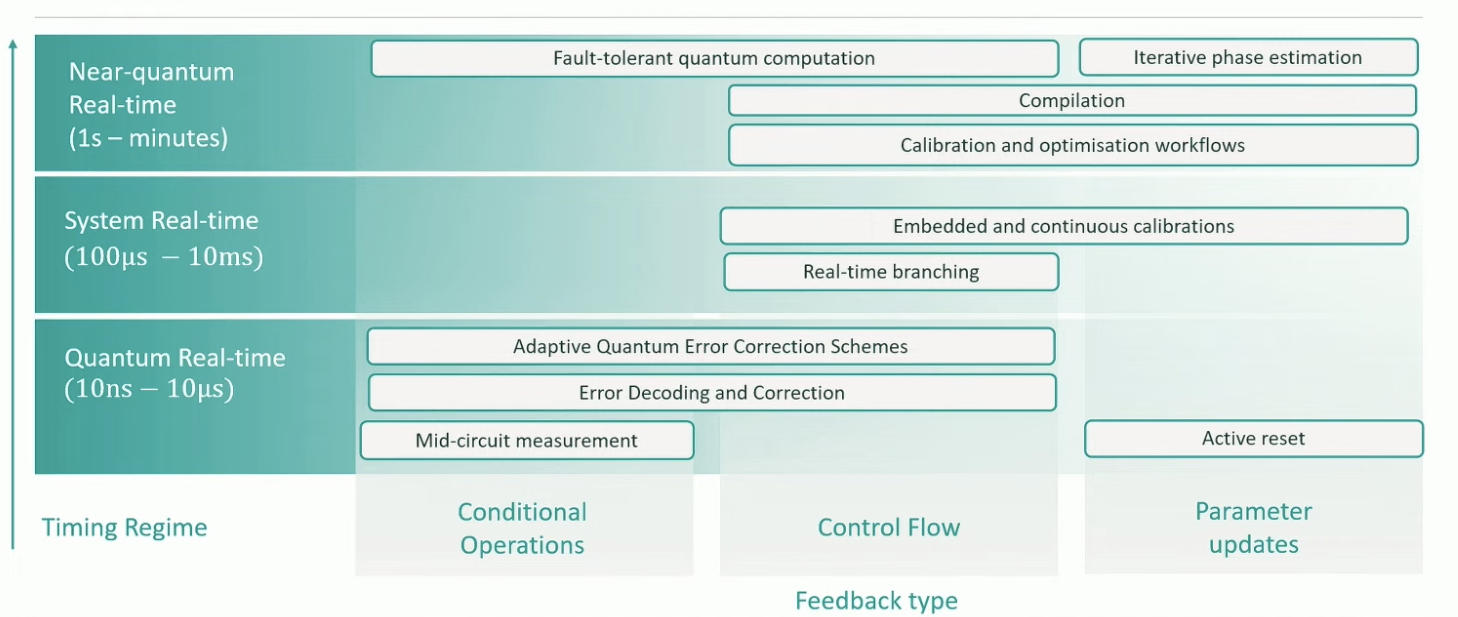
I've picked out some numbers here to show that classical computing is operating at multiple time scales across the quantum computing stack. These numbers are mostly for solid state systems, but it's really just to give you a sense that across the stack, there are multiple different operations happening to do with conditional operations, changes in control flow, updates of the parameters, and so on.
The things that we're trying to implement have different timescales associated with them. For example, solving the decoding problem in quantum error correction needs to happen at a rate of roughly MegaHertz, whereas you can do a large-scale compilation on the time scale of minutes to hours.
There's a bunch of different operations here that all have different timescales. These time scales put serious constraints on what you need that classical compute to be doing.
I'm going to dive into one of these topics to give you a bit of a flavour of what exactly this computer is doing: quantum error correction. This is how we're going to scale the number of error-free operations beyond the thousands that are possible today to the millions and, ultimately, trillions of error-free operations.
Let's just take a quick step back and let me introduce something called the surface code. This has become the dominant way of thinking about quantum error correction. It's a really beautiful example of how we can encode information in quantum systems.

This (above) is a picture of one logical qubit. Each yellow dot is a data qubit. So, these are carrying the quantum state of the computer. The green dots are the ancilla qubits that we add to check if there have been any errors or not. There are two different colours in this patch: the orange and green. These are checking for the two different types of errors that can occur in a quantum system.
I'm just going to focus on one, which is our so-called X errors, or bit flip errors. What do these checks do? You have one orange box, and you essentially check: did I measure a bit flip on any of the four qubits? To find out, you check the parity of those four qubits. If the parity is odd, then the syndrome, so this green qubit, lights up.
In this example, there are two X errors and two of the syndrome bits have lit up. There's one in the middle that's flipped twice, and that's because it still has an even parity. So, there were two errors.
In reality, we don't see this picture when tackling the decoding problem. What we actually see is this picture:

We see the changes in the syndromes. Then, the decoding problem is to, given this information, find out: what was the most likely error?
You can see that there could be different ways to create that same error. In fact, any path from these two endpoints would be a valid explanation for these syndromes. The shortest path, so the one with the fewest number of errors, is the most likely because errors are occurring at a rate of, say, one in 100, one in a thousand. So, fewer errors are more likely than more errors.
So, we're looking to solve the shortest path problem in a grid.
Here comes the test. Now, I've explained how quantum arrow correction works, see if you could solve this problem. Here are the endpoints. If anybody can solve this by the end of this talk, I'll buy you a drink.

The actual problem is much bigger, of course, and we see the syndromes from lots of errors. The task is to figure out, well, how do I best explain this? In other words, given the data, what's the most likely error?
I'm simplifying things again here because, actually, the measurements of the syndromes itself are noisy. There's nothing perfect in this quantum computer.
In fact, the real decoding problem looks more like this:

There's this huge grid of possible syndromes that are all lighting up at a rate of a million times per second. We're getting new data at a rate of a million times per second.
So, the decoding problem with it, which is the classical compute problem for error correction, needs to be at a high accuracy. We need to be good at solving this inference problem, otherwise, we're going to make a mistake.
It also needs high throughput, so there's going to be a lot of data coming out of this quantum computer, and it needs to be low latency.

What I've drawn here (above) is the clock cycle of the quantum computer. Down at the bottom, you have the qubits, you measure this data, solve the decoding problem, and send a correction.
You have to do that between every logical operation on the quantum computer.
So, the speed at which you do this defines the logical clock rate of your quantum computer.
This is a really wonderful classical computing problem that comes from quantum computing.
We've been making a lot of progress in solving this problem over the past 5 to 10 years.
Last year, together with Rigetti, we showed that indeed, you could get this clock cycle working. We embedded the Riverlane decoder inside the control system that was generating the microwave signals for Rigetti to show that this whole cycle worked.
This was a great breakthrough because we showed we could solve this decoding problem faster than the data generation rate. So, we could keep up with the error data, and we could do this very quickly with a latency of around 10 microseconds.
The interesting thing here was we learned an awful lot about embedding this decoding problem within the full quantum computing stack. There's more to do, but there's a huge amount of progress in this space.
The other nice example from last year was the result from Google. This result showed that you could get logical fidelities below physical fidelities. That was a huge achievement.
One of the interesting things here is the way that the Google team approached this, making use of extensive software calibration. There are imperfections in the fabrication of the superconducting chip, and Google is very good at software development, and adds this software layer on top to account for that or to correct for that. There's a huge amount of calibration that goes into this result.
This is another example where classical computers are used extensively in quantum computing.
There has also been a huge amount of progress at the qubit level for quantum computers.

On the left-hand side of these plots, you can see the physical fidelities of multiple different qubit modalities over the past two decades.
One of the interesting things here is that a lot of this has been done by repurposing stuff from other industries.
Most of the control electronics are essentially built by Xilinx to develop 5G base stations. It's not built for quantum computing.
What excites me about the next decade in quantum computing is the specialisation, the building of components that then continue to drive forward quantum computing.
The second point here is that the roadmaps of multiple companies in this space get us to around 10,000 physical qubits over the next few years. Together with error correction, this means we can build the first error-corrected quantum computer. This will be called the MegaQuOp, so one million quantum operations.
I thought it was interesting just to compare the computational power of that MegaQuOp quantum computer with an equivalent supercomputer.

On the left-hand side, you can see the MegaQuOp specs, where a MegaQuOp is one million error-free operations. That's around 1,000 to 10,000 times more than current quantum computers have, and it would have around 100 logical qubits.
Now, if you wanted to simulate that quantum computer just very directly using the best-known simulation method, you would need on the order of a billion trillion GPUs.
In other words, it would be impossible to build such a system. This will be the first quantum computer that nobody can simulate. We saw an interesting example in an earlier talk about the first application for that. I think there is a huge potential to come up with new applications or more applications for that machine.
The MegaQuOp is also the first step in a much longer journey. Having built the MegaQuOp quantum computer, the next generation will be the GigaQuOp and then the TeraQuOp.
As we increase the number of quantum operations that are possible, then the application space will grow enormously.
This journey will be one of both science and engineering. And the third thing that will enable this journey is the specialisation of key components within the quantum computing stack – with people dedicating resources to solving particular parts of the whole problem for quantum computing. Thank you.