

Imagine trying to find a needle in a haystack while being blindfolded. Then, someone offers to remove the blindfold. Would you do it?
Now, imagine trying to improve the error correction on your quantum chip without any error budgeting. Then, someone offers to give you an easy-to-use and fully implemented error-budgeting procedure for free. Would you take the offer?
The answer to both questions should be ‘yes’.
This post dives into the crucial concept of error budgeting in Quantum Error Correction (QEC), explaining what it is, why it's vital, how it works, and how a new open-source implementation makes it accessible (and free) to everyone through the Deltakit library.
What is error budgeting?
Before defining error budgeting, let's introduce a few important metrics in Quantum Error Correction (QEC):
· The logical error probability: This is one of the most critical metrics in QEC, representing the probability of an error even after applying the error-correction protocol. It dictates how many operations can probably be executed reliably. However, this metric has a drawback: it depends heavily on the size of the quantum computation being considered (e.g., Shor's algorithm vs. a simple memory experiment).
· ε: the logical error probability per round: To address the computation dependency, researchers developed ε, the logical error probability per round for a given distance d. Most QEC codes require repeating operations (rounds) for effective error accounting. This metric is significantly better when comparing performances as it can be considered computation-independent for a given hardware and code implementation.
· Λ: the error suppression factor: We can go even further with a distance-independent metric called Λ. This is the multiplicative factor by which the error probability per round is reduced when you increase the code-distance by 2 (i.e., when you can correct one more physical error). Mathematically:
Λ = Ɛ(d) / Ɛ(d+2)
This metric depends on the implemented code, its practical implementation, and the hardware error rates. Crucially, for a specific hardware, Λ allows for a direct comparison of the efficiency of different error-correction code implementations.
So, where's the budget?
A "budget" is typically defined by a quantity you want to minimise, which can be expressed as a sum of independent contributions. In our case, we want to minimise ‘1/Λ’.
Research has shown that 1/Λ can be approximated as a linear sum of contributions from various physical error mechanisms (e.g., two-qubit gate error rates, idling error rates, measurement errors, leakage).
Error budgeting is, therefore, the process of computing these individual contributions to 1/Λ.
Why is an error budget essential?
The need for error budgeting stems from a fundamental principle in optimisation: BENCHMARK IT!
As I've advocated for years, whether optimising code or QEC, you cannot know for sure what part of your system is problematic without robust benchmarking. Guessing might sometimes be right, but certainty comes only from measurement and analysis.
For quantum error correction, we strive to minimise 1/Λ to achieve more efficient error correction. An error budget acts as this crucial benchmark, showing exactly where to focus optimisation efforts to achieve the greatest impact. This has important implications for all those working in quantum computing:
· For hardware manufacturers: Error budgeting makes it easy to identify the main sources of errors impacting logical error rates. This clarity allows for better planning of hardware improvements and provides a clear idea of the return on investment (ROI) for those improvements.
· For QEC researchers and implementers: It provides a straightforward way to assess the impact of common noise sources on new QEC codes. This allows for designing more resilient codes or tailoring existing ones to specific architectures with varying noise characteristics.
In other words, error budgeting is a crucial tool, enabling quick understanding of bottlenecks in a given code or hardware. The Deltakit implementation, being the first open-source one, is designed to significantly fasten these improvement cycles across the community.
Get started with Deltakit
Read on for a deeper scientific explanation
Computing an error budget: Technical insights
Calculating an error budget primarily involves computing the gradient of 1/Λ with respect to the error rate of each physical error mechanism. The two main approaches differ based on whether a first-order or second-order approximation of 1/Λ is used.
The primary challenge here is that 1/Λ is a "noisy" function. The computation chain becomes:
· 1/Λ requires to compute Λ.
· Λ requires to compute εd for at least two distances.
· εd requires to find the logical error probability for different numbers of rounds.
· The logical error probability estimation relies on Monte Carlo sampling (often with tools like stim), which inherently introduces uncertainty.
This uncertainty propagates up to the estimation of 1/Λ, making its values inherently noisy. Traditional numerical methods for gradient computation, like standard finite differences, struggle with noisy data.
The solution implemented involves using multiple values of 1/Λ evaluated at different noise strengths to approximate 1/Λ with a polynomial.
Computing the gradient of this polynomial at the point of interest significantly reduces the numerical sensitivity to uncertainties in the gradient estimation procedure and, crucially, allows for the computation of the standard deviation of the gradient estimation, providing confidence intervals for the results.
Diving into the weeds of quantum error-correction metrics, numerical analysis, and error propagation for standard deviations was both fun and invaluable.
This is because, once computed, an error budget provides actionable insights.
Let’s say that you estimated the error budget of your implementation of the rotated surface code on a specific hardware with several noise sources and obtain the following budget:
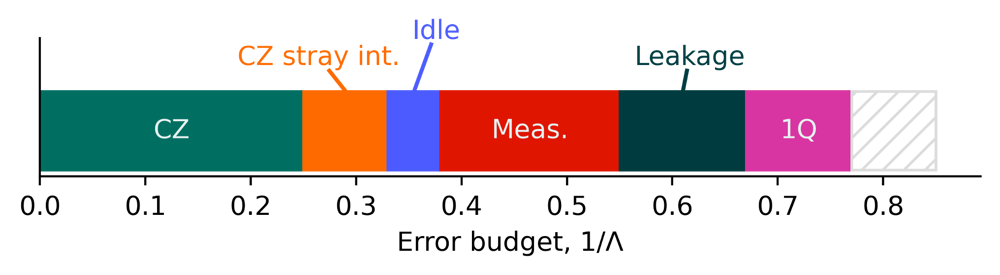
This image above encapsulates a lot of information about your actual error-correction performance and how to improve it.
The right-most area dashed in white represents the “excess” noise, which is the difference between the value computed on the real hardware and the value obtained by combining each individual contribution.
The two-qubit error-rates account for ≈ 0.32 of the total budget, which is 0.32/0.85 ≈ 38% of the total budget. That means that dividing your two-qubit error-rate by 2 would reduce your 1/Λ by ≈ 38/2 = 19% and so increase your Λ by ≈ 23%.
Reducing the idle noise would probably not have a large impact on your error-correction performance because idling noise is only ≈ 6% of the budget.
In conclusion
A QEC team without error budgeting is like a carpenter without a band saw: unable to efficiently perform their job. Trying to improve your error correction performance without it is akin to searching for that needle in a haystack while blindfolded – it's possible, but incredibly inefficient.
Thanks to the new open-source implementation in Deltakit, it is now easy to perform error-budgeting estimations for your particular noise model, QEC code, or its implementation.
By leveraging these new capabilities, you can tailor your noise models to your hardware and improve your logical error probabilities.
If you’d like to find out more, you can get started with Deltakit here.